flowchart LR
   id1[SQL text] --> |SQL parser| id2[SQL statement]
   id2 --> |Query planner| id3[Logical plan] --> |Query optimizer| id4[Optimized logical plan] --> |Physical planner| id5
   id5[Physical plan] --> |Execution| id7[Output]
Preface
A database can be complex; it involves almost all aspects (research communities) of computer science: PL (programming language), SE (software engineering), OS (operating system), networking, storage, theory; more recently, NLP (natural language processing), and ML (machine learning). The database community is centered around the people interested in making the database (the product) better instead of pure intellectual/research interests; it is, therefore, a practical and multi-disciplinary field. This makes databases awesome but also hard to learn.
As complex as it is, the boundaries of the building blocks within a database are clear after decades of research and real-world operations. The recent (and state-of-the-art) Apache DataFusion project is a good example of building a database using well-defined industry standards like Apache Arrow, and Apache Parquet. Without home-grown solutions for storage and in-memory representation, DataFusion can be comparable or even better than alternatives like DuckDB.
This document aims to explain these well-defined boundaries, namely, how query engines (i.e., OLAP) transform a plain SQL query into the results we want, how every step works, and how they are connected.
Note
This is a blog post I hoped I knew when I was younger.
I aim to make multi-year efforts to edit and improve it as I learn more about databases. I sometimes dreamed that this post could evolve to be the database equivalent of the OSTEP book (it might be too ambitious, though).
Section 1: End-To-End View
Input
Table definition
We have the following two tables (adapted from TPC-H spec): lineitem and orders. The lineitem defines the the shipment dates, while the order defines order details.
erDiagram
  lineitem {
      int l_orderkey
      int l_linenumber
      date l_shipdate
      date l_commitdate
      date l_receiptdate
      string l_shipmode
      string l_comment
  }
  orders {
      int o_orderkey
      date o_orderdate
      string o_orderpriority
      string o_clerk
      string o_comment
  }
SQL query
Let’s say we have this simple query (adapted from TPC-H query 5), which finds the l_orderkey, l_shipdate, and o_orderdate of orders that were placed in 1994.
SELECT
    l_orderkey, l_shipdate, o_orderdate
FROM
    orders
JOIN
    lineitem ON l_orderkey = o_orderkey
WHERE
    o_orderdate >= DATE '1994-01-01'
    AND o_orderdate < DATE '1995-01-01';
Output
The query is pretty simple; it joins two tables on the order key and then filters the results based on the order date. If everything goes well, we should get results similar to this:
+------------+------------+-------------+
| l_orderkey | l_shipdate | o_orderdate |
+------------+------------+-------------+
| 1          | 1994-06-01 | 1994-05-01  |
+------------+------------+-------------+
Section 2: Parsing
I skipped it for now as it is mostly orthogonal to the data system pipelines.
Input
The SQL query text.
Output
Structured statement from the SQL (significantly simplified for brevity):
from: [
  TableWithJoins {
    relation: Table {
      name: ObjectName([
        Ident {
          value: "orders",
          quote_style: None,
        },
      ]),
    },
    joins: [
      Join {
        relation: Table {
          name: ObjectName([
            Ident {
              value: "lineitem",
              quote_style: None,
            },
          ]),
        },
        join_operator: Inner(
          On(
            BinaryOp {
              left: Identifier(
                Ident {
                  value: "l_orderkey",
                  quote_style: None,
                },
              ),
              op: Eq,
              right: Identifier(
                Ident {
                  value: "o_orderkey",
                  quote_style: None,
                },
              ),
            },
          ),
        ),
      },
    ],
  },
],
selection: Some(
  BinaryOp {
    left: BinaryOp {
      left: Identifier(
        Ident {
          value: "o_orderdate",
          quote_style: None,
        },
      ),
      op: GtEq,
      right: TypedString {
        data_type: Date,
        value: "1994-01-01",
      },
    },
    op: And,
    right: BinaryOp {
      left: Identifier(
        Ident {
          value: "o_orderdate",
          quote_style: None,
        },
      ),
      op: Lt,
      right: TypedString {
        data_type: Date,
        value: "1995-01-01",
      },
    },
  },
),
Section 3: Query Planning
Input
The query statement from the last step.
Output
The logical query plan is something like this:
Projection: lineitem.l_orderkey, lineitem.l_shipdate, orders.o_orderdate
  Filter: orders.o_orderdate >= CAST(Utf8("1994-01-01") AS Date32) AND orders.o_orderdate < CAST(Utf8("1995-01-01") AS Date32)
    Inner Join:  Filter: lineitem.l_orderkey = orders.o_orderkey
      TableScan: orders
      TableScan: lineitem
Plot it as a tree.
Logical vs physical.
Todo: describe why we must distinguish between physical and logical plans.
Section 4: Query Optimizing
Input
The (unoptimized) logical plan from the last step.
Output
An optimized logical plan.
Projection: lineitem.l_orderkey, lineitem.l_shipdate, orders.o_orderdate
  Inner Join: orders.o_orderkey = lineitem.l_orderkey
    Filter: orders.o_orderdate >= Date32("8766") AND orders.o_orderdate < Date32("9131")
      TableScan: orders projection=[o_orderkey, o_orderdate], partial_filters=[orders.o_orderdate >= Date32("8766"), orders.o_orderdate < Date32("9131")]
TableScan: lineitem projection=[l_orderkey, l_shipdate]Note the difference between an unoptimized and an optimized plan! The Filter has been pushed down to lower-level nodes. Part of the projection has been embedded in the TableScan.
Section 5: Physical Planning
Input
A logical plan.
Output
A physical plan. Unlike logical plans, physical plans are more concrete about what to do; here’s an example:
Physical plan:
ProjectionExec: expr=[l_orderkey@1 as l_orderkey, l_shipdate@2 as l_shipdate, o_orderdate@0 as o_orderdate]
  CoalesceBatchesExec: target_batch_size=8192
    HashJoinExec: mode=Partitioned, join_type=Inner, on=[(o_orderkey@0, l_orderkey@0)], projection=[o_orderdate@1, l_orderkey@2, l_shipdate@3]
      CoalesceBatchesExec: target_batch_size=8192
        RepartitionExec: partitioning=Hash([o_orderkey@0], 8), input_partitions=8
          CoalesceBatchesExec: target_batch_size=8192
            FilterExec: o_orderdate@1 >= 8766 AND o_orderdate@1 < 9131
              RepartitionExec: partitioning=RoundRobinBatch(8), input_partitions=1
                CsvExec: file_groups={1 group: [[Users/xiangpeng/work/coding/db-ml/bin/example-data/orders.csv]]}, projection=[o_orderkey, o_orderdate], has_header=true
      CoalesceBatchesExec: target_batch_size=8192
        RepartitionExec: partitioning=Hash([l_orderkey@0], 8), input_partitions=8
          RepartitionExec: partitioning=RoundRobinBatch(8), input_partitions=1
            CsvExec: file_groups={1 group: [[Users/xiangpeng/work/coding/db-ml/bin/example-data/lineitem.csv]]}, projection=[l_orderkey, l_shipdate], has_header=true
We can also plot a physical plan to a tree graph:
Note
Note that a physical plan has much more details than a logical plan; it contains everything needed to execute the query!
(Optional: we often have physical optimizers that optimize on a physical plan. Omitted here for simplicity)
Section 6: Query Execution
Input
A physical plan
Output
The final output is like this:
+------------+------------+-------------+
| l_orderkey | l_shipdate | o_orderdate |
+------------+------------+-------------+
| 1          | 1994-06-01 | 1994-05-01  |
+------------+------------+-------------+
Execution order
The simplest execution model is pull-based execution, which implements a post-order traversal of the physical plan. For a tree (like blow), we get a traversal order of D -> E -> B -> F -> G -> C -> A: 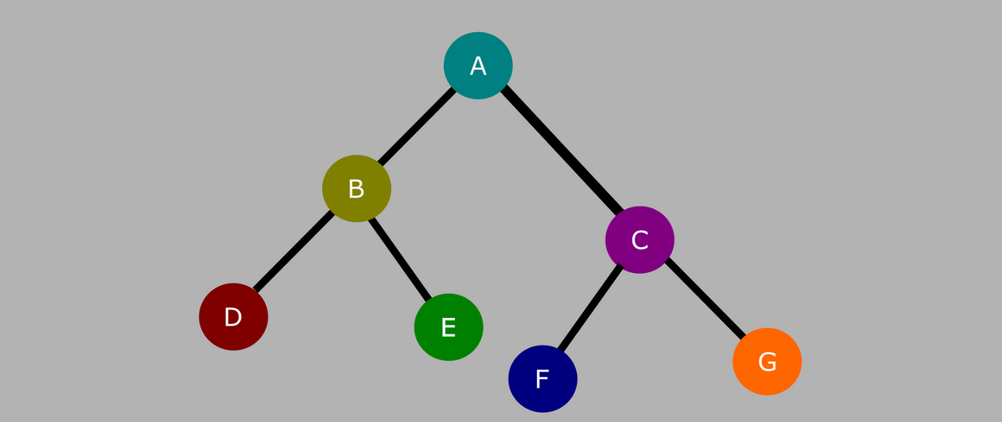
Applying our physical graph above, we get an execution order of:
The RepartitionExec and CoalesceBatchesExec are executors that partition the data for multi-thread processing (based on the Volcano execution style).
A simplified, single-threaded, no-partitioned execution order would be:
graph LR;
    e1["CsvExec (orders.csv)"] --> FilterExec
    FilterExec --> e2
    e2["CsvExec (lineitem.csv)"] --> HashJoinExec
    HashJoinExec --> ProjectionExec
Reading from disk
CSV files are row-based, and we read them row by row, it is efficient when we frequently need to read the whole row. However, modern data analytic workloads do not always need to read the whole row; they often only need to read a subset of columns. In our example above, we only need to read l_orderkey, l_shipdate, o_orderdate, o_orderkey from the tables. If using a row-based file format (like CSV), we need to load all columns into memory, which is inefficient. Column-based file formats (like Apache Parquet) can be more efficient in this case.
See the Parquet pruning in DataFusion for more details.